Lab 5 Working with Spreadsheets

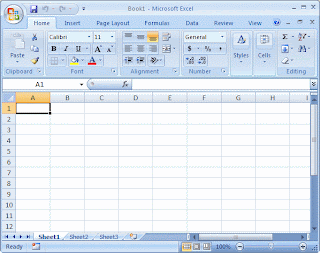
The main purpose of this lab was to get students more familiar and comfortable with using Microsoft Excel. All we needed to preform this lab was a computer with Excel and Graphical Analysis.

 We were instructed to create a spreadsheet that calculated the values of the function
f(x) = A sin(Bx+C). The initial values were A = 5, B = 3, C = Pi/3. We selected a seperate column for each of these initial values. The column for A was named amplitude, the column for B was named Frequency, and the column for C was named Phase. We then chose a column for the values of X. We called that column radians, and typed in values of X from 0-10 radians in steps of .1 radians (101 readings). Finally we created a column for the f(x) values. Once we generated all the values we were told to print out the fiirst 20 readings and then to print out a spreadsheet of the formulas by pressing CTRL~.

 

 Once we had the desired readings, we copied both columns ( x and f(x)) and pasted them into Graphical Analysis. A graph came up and we had to choose the right ANALYZE/CURVE FIT to find a function that best fit the data. The values of A, B, and C were all the same from our previous spread sheet.

We then made a different spreadsheet that calculated the position of a freely falling particle as a function of time. This time our constants were acceleration of gravity, initial velocity, and initial position in time increments of .2s. We started off with g (C) = 9.8 m/s^2, Vo (B) = 50 m/s, Xo (A) = 1000m, and delta t = .2 s. Our function looked something like this f(x) = A + Bx + 1/2Cx^2. We repeated the steps above by printing out the first 20 readings and first 20 forumlas.

We then copy pasted all the values into a Graphical Analysis and printing out the graph and comparing the Curve Fit to our original values. Everything was smooth as water. We chose the quadratic fit and all the values were the same as our originals.

In conclusion I was amazed by the consistancy and lack of error output of the computer and how the excel sheet did amazing calculations. I was familiar with excel, in making charts and have used it a couple times on recording tax incomes but never this thoroughly with physics. It was really cool to see another source of physics being put to work with the free fall diagram, and how precise and accurate the computer was with all the readings and the graphs and how it all worked out together. I must say I did not expect this at all when we first started the lab, and was very nervous half way through our lab because I was worried both me and my partner wouldn's comprehend all the tasks at hand. Luckily for us we teamed with another group who knew what they were doing and they walked us through the steps and didn't get frusturated when we asked them to repeat a step or to reexplain things we didn't catch the first time. In all this lab was very beneficial in the physics world as to charting out data and using two different computer programs to explain more physics. I recommend this lab for years to come.

Lab 4 Vector Addition of Forces

This lab was by far the most conceptual. The purpose of this lab was to study vector addition by graphical means and by adding components. A circular force table was used to check our results. To do this lab we needed a protractor, ruler, mass holders, masses, circular force table and four pulleys.

 The lab started off with the instructor giving each group three masses (which represented magnitude of a vector) and an angle to go with each one. We were instructed to use 100 grams at 0 degrees, 200 grams at 71 degrees, and 160 grams at 144 degrees.

We were told, as our first step to take a ruler, graphing paper, and protractor and to add all these vectors by hand. We were instructed to draw the vectors to scale, having 1 cm=20 grams and to find the resultant vector.

Here we found a resultant vector, we called R, to be 284 grams and 83 degrees. Then we were told to make a second vector diagram, this time using components of each vector to to draw the resultant vector.

Now came the fun part, putting our calculations to work. We mounted three pulleys on the edge of the force table at the angles given to us. Then we attached the strings from the center ring so that they each ran over the pulley and attached a mass holder to the opposite end of it.

We were told to hang the appropriate mass at the three appropriate angles and to set up a fourth mass at a fourth angle to cause equalibrium. This fourth angle happened to be 180 degrees opposite the resultant vector found earlier in our calculations.

We were then told to visit a website, as seen above, and insert all of our data in order to form a resultant vector. The scale on the website is in incriments of 10. We found out that we were correct. There were no error in our calculation and the computers.

The only real calculation  came from adding components of vectors to find the resultant vector.We had to find each x component of the given vectors and each y component of the given vectors. Once we did that we added all the x components and all the y components and got our resultant vector components. From these two values we could use the pythagreon theorom to find the magnitude of our resultant vector, and to find the angle it made we used the inverse tangent property of the y component divided by the x component

Angle	Magnitude	X Component	Y Component
0	100	100*cos(0) = 100	100*sin(0) = 0
71	200	200*cos(71) = 65.1	200*sin(71) = 189
144	160	160*cos(144) = -129	160*sin(144) = 94.0
		X Component Result	Y Component Result
		36.1	283
		Magnitude Result	Theta Result
		((36.1^2)+(283^2))^.5 = 285.3	Tan^-1(283/36.1) = 82.7

In this lab I learned that if all of our vectors are added up, 180 degrees off the resultant vector, with same magnitude would balance it out on a circular force table. I had some idea that this would work out because I am in calculus 3c, and that class is all about vectors. The error came from using protactors and rulers to estimate the resultant vector of adding the three given vectors. There was also error in adding weight to the pullies. I even saw one of the weight say 49.5 on it while having 50 grams engraved in it. It's also possible for the pullies to have grease spots or not such smooth rotation after being used over the years hence adding more marginal error. Another place we could find error was lining up the pullies and the right degree on the circular force table, both human error and significant error played a major role.

Lab 3 Acceleration of Gravity on an Inclined Plane

In this lab we attempted to find the acceleration of gravity on an object. We started with a frictionless track, a car for the track, a couple blocks of wood (to shift incline), and a device that measured position vs time. We connected this device to a computer and had a program draw us graphs of position vs time and plot its velocity versus time as well.

 The picture above shows roughly all the equipments needed to do this lab.

From there we inclined the track at an angle of 2.40 degrees above the horizontal(note error). We did this by measuring the height on both sides of the track and using the pythagrean theorem  We took many trials until we got the best three possible results. The computer program had a property that gave us a linear fit. We used the linear fit on two parts of the velocity graph in order to get an average acceleration reading.

 

 

After we had three reasonable trials for the first heigh (angle), we changed the hieght of the track again. This time we raised one side a bit higher and developed an angle 4.69 degrees above the horizontal. We did a few more trials until we got the desired graphs we were looking for.

 We were given an equation for gravity. The equation stated, the average acceleration divided by sine of the angle theta would give us acceleration due to gravity. The percent error was calculated by subtracting the final answer from the actual gravity, taking the magnitude of that value, and dividing it by the actual value and multiplying it by 100.

	Height	Length	Angle	Accel 1	Accel 2	Avg Accel	Gravity	% Error
One	9.55 cm	228 cm	2.4	.4021 m/s/s	.3205 m/s/s	.3613 m/s/s	8.62 m/s/s	12.1
Two	9.55 cm	228 cm	2.4	.3921 m/s/s	.3186 m/s/s	.3554 m/s/s	8.49 m/s/s	13.5
Three	9.55 cm	228 cm	2.4	.4000 m/s/s	.3135 m/s/s	.3568 m/s/s	8.52 m/s/s	13.2
Four	18.65 cm	228 cm	4.69	.7903 m/s/s	.6956 m/s/s	.7430 m/s/s	9.09 m/s/s	7.38
Five	18.65 cm	228 cm	4.69	.8077 m/s/s	.7118 m/s/s	.7598 m/s/s	9.29 m/s/s	5.28
Six	18.65 cm	228 cm	4.69	.7959 m/s/s	.7100 m/s/s	.7530 m/s/s	9.21 m/s/s	6.13

In conclusion we found that sin theta times gravity gave us the acceleration of the car. It was very interesting that the lab proved the books point. The reasons we didn't come too close to the reading seemed, for one, was lack of track space. It seems as though the track cars that were at a higher angle came closer to the actual value of gravity because it moved faster, over coming and negligable force of friction on the track. Other than that the hieght measurements with the meter stick could throw off the reading a bit. The unlevel surfaces of the table could interfere with our readings. I'm still very curious to know why on the steeper incline we were more accurate. I was pleased to see all readings were very precise, shows that we were doing the experiment correctly.